How I Turned a 100 ms Problem into a Microsecond Query with AI-Assisted Performance Engineering

A real Hungarian-lottery problem, two complete solutions with the actual Go on the table, and the honest story of how AI helped collapse latency from a 100 ms budget to ~1.5 microseconds — not in one prompt, but one disciplined iteration at a time.

One of the most useful ways I have found to work with AI on a performance problem is not to ask:

“Can you optimize this code?”

but instead to ask:

“What work can be moved out of the critical path?”

That single question often rewrites the entire architecture. This article is about a problem that began with one ordinary line in a spec — maximum acceptable query latency: 100 ms — and ended somewhere I did not expect.

The job was to report winner counts for a lottery-like system with up to 10 million players. The final results landed like this:

100 ms budget
        ↓
12 ms   optimized parallel scan      (ordinary systems engineering)
        ↓
1.5 µs (0.0015 ms)  indexed O(1) query           (AI-assisted redesign)

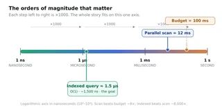
Put another way: the budget was 100 ms = 100,000,000 ns. The final query latency was about 1,500 ns — roughly 66,000× under budget. But the final number is not the interesting part. The interesting part is how AI can help decompose a problem into known building blocks that snap together into something dramatically faster — and how much human steering that took.

Before we go anywhere, it helps to fix the scale we are talking about, because the difference between a millisecond and a microsecond is the difference between “fast enough” and “effectively free.”

The relationship between the units is worth committing to memory — performance work lives and dies on knowing which unit you are in:

UNIT          SYMBOL   SECONDS        vs. NEXT UNIT     EVERYDAY FEEL
─────────────────────────────────────────────────────────────────────────
second         s       1              —                 a slow page load
millisecond    ms      0.001          1 s   = 1,000 ms  a snappy API call
microsecond    µs      0.000001       1 ms  = 1,000 µs  a few memory reads
nanosecond     ns      0.000000001    1 µs  = 1,000 ns  one CPU instruction
─────────────────────────────────────────────────────────────────────────
This project:  100 ms budget  →  12,000 µs scan  →  1.5 µs indexed query
               100,000,000 ns →  12,227,000 ns   →  ~1,500 ns

The Hungarian Lottery problem

The rules are simple:

• Each player chooses 5 distinct numbers from 1 to 90.
• Later, the lottery draws 5 distinct winning numbers.
• A player wins if they match exactly 2, 3, 4, or 5 numbers.
• At peak load there can be around 10 million players.
• After the draw, the system must immediately report the winner counts.

The required output, after each draw, answers four questions: how many players matched exactly 2 numbers, exactly 3, exactly 4, and exactly 5?

At first glance this looks trivial — it is a counting problem. But performance engineering starts the moment someone adds a latency requirement. With maximum response time after the draw: 100 ms in the spec, the question quietly changes. We stop asking “can we count the winners?” and start asking the only question that matters at scale:

How much work must happen after the winning numbers are known?

That distinction leads to two very different implementations: a scan-based solution optimized for simplicity, low memory, and cache efficiency; and an indexed solution optimized for extremely low post-draw latency. Both are useful. Both are worth understanding. And the gap between them is where this story lives.

Understanding the shape of the problem

Performance-heavy problems are rarely solved by one trick. Most of the time, the real work is understanding the shape of the problem before writing any code. I try to answer a small set of questions first:

• What is known ahead of time?
• What must be answered immediately?
• What is the true critical path?
• Where is the bottleneck — CPU, memory bandwidth, allocation, I/O, synchronization, or algorithmic complexity?
• What tradeoff are we willing to make between memory, preprocessing time, and query latency?

For the lottery, the answers are clarifying. The tickets are known before the draw; the winning numbers are only known after. The critical path — the part a human is actually waiting on — is the post-draw report; everything else is preparation we can do on our own schedule. So the right question is not “how fast is the whole program?” but “how fast is the part users are waiting for?”

Thinking like an AI performance agent

When I work with AI on optimization problems, I try to hand it constraints instead of implementation details. Something like this:

Goal:        Answer winner counts after the draw.
Constraint:  Maximum latency 100 ms.
Dataset:     Up to 10 million tickets.
Allowed tradeoffs:
             more preprocessing,
             more memory,
             lower query latency.
Question:    What work can be moved before the draw?

That framing naturally produces two architectures: scan everything after the draw, or precompute enough that the draw becomes almost free. The second option is where things get interesting — but I want to be honest up front about the order of events. I did not arrive at the fast solution by typing one clever prompt. I arrived at a solid, ordinary solution first, by hand, and only then used AI to attack the part that ordinary engineering could not improve.

The key idea: split the problem into phases

Because the tickets are known before the draw and the winning numbers are not, the system splits naturally into two phases:

For performance-heavy problems, this separation is often more important than the algorithm itself. A system that does more work before the draw and very little after can beat one that starts quickly but scans everything while the clock is running. This is one of the most important patterns in our field: move work from the critical path into a preparation phase. Search engines do it with inverted indexes, databases with secondary indexes, compilers with intermediate representations, recommendation systems with precomputed features. The lottery is no different.

High-level architecture

The final design supports two execution modes that share the same front end. Input is parsed in parallel into a compact packed representation, and from there the data feeds either a scan path or an indexed path:

The scan mode met the latency target comfortably. The indexed mode essentially eliminated query latency altogether. We will build both — and, conveniently, both satisfy the same one-line Go signature, so the rest of the program is written against the interface and the algorithm is chosen at startup with a flag:

type winnerCounter func(d1, d2, d3, d4, d5 int) (w2, w3, w4, w5 int)

// ./lottery -mode scan   input.txt   → O(N) per draw, lower memory
// ./lottery -mode indexed input.txt  → O(1) per draw, default

That symmetry is not just tidy; it is what lets the slow path verify the fast one later.

Solution 1 — the cache-friendly scan (12 ms, and no AI required)

I want to be clear: there is no AI magic in this section. The 12 ms result came from ordinary, disciplined systems engineering — the kind any performance-minded engineer can do with a profiler and some patience. That matters, because it sets the bar the AI-assisted solution had to beat.

The scan solution is the simplest correct approach. Load all tickets into memory, then for each draw, scan every ticket and count matches:

for each ticket:
    matches = count numbers that appear in the draw
    if matches == 2: winners2++
    if matches == 3: winners3++
    if matches == 4: winners4++
    if matches == 5: winners5++

The complexity is O(N) per draw. For 10 million players that sounds expensive, but the constants are tiny — and data layout is where the win comes from.

Compact representation

Instead of storing tickets as objects, structs, maps, or nested slices, store them as one flat byte array:

tickets []byte        // player i occupies tickets[5*i : 5*i+5]

So the memory layout is just numbers, back to back, with nothing in between:

Player 0        Player 1        Player 2
┌─────────────┐ ┌─────────────┐ ┌─────────────┐
│ n n n n n   │ │ n n n n n   │ │ n n n n n   │ ...
└─────────────┘ └─────────────┘ └─────────────┘

Flat memory: [n0 n1 n2 n3 n4][n0 n1 n2 n3 n4][n0 n1 n2 n3 n4]...

With one byte per number, 10 million tickets pack into about 10,000,000 × 5 = 50 MB, and a modern CPU streams through 50 MB of contiguous memory surprisingly quickly. (The raw text file is closer to 145 MB — more on how we avoid copying that later.) The advantages stack up: no per-ticket allocation, no pointer chasing, a compact footprint, sequential access, cache-friendly scanning, and trivial chunking across workers.

“For performance-heavy code, data layout is part of the algorithm. A theoretically simple algorithm with good locality routinely beats a cleverer algorithm implemented with poor locality.”

The hot loop: a 91-byte table that lives in L1

For each draw, build a tiny membership table — one byte per possible number — and mark the five that were drawn. At 91 bytes it stays resident in L1 cache, so every lookup is essentially free. Counting a player then collapses to five indexed reads and an increment: no set intersection, no map lookup, no sorting, no allocation. Here is the actual hot loop, lifted straight from the source:

var isDrawn [maxNumber + 1]byte            // 91 bytes — resident in L1
isDrawn[d1], isDrawn[d2], isDrawn[d3], isDrawn[d4], isDrawn[d5] = 1, 1, 1, 1, 1

// each worker walks its own slice of players into a private histogram:
for player := chunkStart; player < chunkEnd; player++ {
    o := player * 5
    m := isDrawn[t[o]] + isDrawn[t[o+1]] + isDrawn[t[o+2]] +
         isDrawn[t[o+3]] + isDrawn[t[o+4]]   // m is 0..5
    histogram[m]++                           // buckets 2..5 are the answer
}

That is the entire computation: a branch-free sum of five bytes and one array bump, ten million times — the kind of work a CPU chews through without complaint.

Parallel scanning

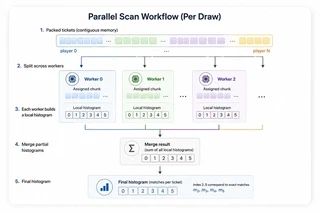
The scan splits cleanly across CPU cores. Each worker processes a contiguous range of players and keeps a private histogram, so there is no locking in the hot loop:

Packed tickets
┌───────────────────────────────────────────────┐
│ player 0 ............................. player N │
└───────────────────────────────────────────────┘
       │              │              │
       ▼              ▼              ▼
┌────────────┐  ┌────────────┐  ┌────────────┐
│ Worker 0   │  │ Worker 1   │  │ Worker 2   │
│ hist[0..5] │  │ hist[0..5] │  │ hist[0..5] │
└─────┬──────┘  └─────┬──────┘  └─────┬──────┘
      └───────────────┼───────────────┘
                      ▼
              ┌──────────────┐
              │ Merge result  │
              └──────────────┘

The theoretical complexity stays O(N), but practical latency approaches O(N / p) where p is the number of cores. Better still, every worker walks a contiguous, predictable region of memory — exactly the access pattern hardware prefetchers love.

Result: 12 ms

On a deliberately constrained box — 4 logical CPUs, 4 GB RAM — the scan implementation handled 10 million players with an average draw latency of about 12.2 ms. Against a 100 ms budget, that is already ~8× faster than required. Mission accomplished. Or so it seemed.

Why keep scan mode at all?

It is simple, memory-efficient, easy to debug, and easy to trust. It makes a perfect correctness baseline, shines when memory is tight or draws are rare, and — as we will see — can verify the fast solution. Before building a complex optimization, build the simplest version that is fast enough to measure: sometimes it is already good enough, and always it tells you where the real bottleneck is.

Asking AI a better question

With 12 ms in hand, the lazy follow-up would have been “Can this be faster?” AI is happy to answer that — tighter loops, SIMD, chunk-size tuning — and you claw back a few percent. Instead I asked a structurally different question:

Can the query become independent of the number of players?

That changes everything. A few percent is optimization; independence from N is a different runtime model. The answer turned out to be yes — and the resulting architecture is not new mathematics but a composition of several classical ideas. Composing them correctly, in code, at 1.5 µs, was not a one-shot prompt.

The AI collaboration was iterative, not one prompt

This is the part most “I used AI to 1000× my code” stories quietly skip. The reframing question opened the door, but walking through it took several rounds of precise instruction, architectural constraints, and — above all — measurement and verification at every step. Here is the honest iteration log.

Iteration 1 — the first design was correct and slow

Asked to make the query independent of N, the model proposed precomputing combination frequencies and answering via lookups. Good instinct — but its first implementation keyed everything on hash maps: map[pair]int, map[triple]int, and so on. Correct, yet heavy: hash computation on the hot path, bucket overhead, pointer chasing, GC pressure, unpredictable latency. I gave it a hard constraint: no hashing on the query path, no per-item allocation.

Iteration 2 — dense arrays demand a bijection

Removing maps means storing counts in flat arrays, which forces a new sub-problem: every combination needs a deterministic integer index. I pinned it precisely — “map each sorted k-combination to a unique index in [0, C(90,k)), allocation-free” — and the model reached for the combinatorial number system (combinadics). Two details were non-negotiable: convert numbers to zero-based first, and precompute the binomial coefficients with Pascal’s recurrence so C(n,k) is never recomputed in a loop.

Iteration 3 — the inflated-counts bug (caught by the baseline)

The first end-to-end indexed run produced numbers that were obviously too large — the single most important moment in the project, and I only caught it because the scan baseline gave me the invariant scan(draw) == indexed(draw), which failed. The cause is a classic trap: subset totals are not exact-match counts. A 5-match ticket is also counted inside every pair, triple, and quadruple total. I asked the model to derive the correction rather than patch it, pinning the contribution table (a 4-match ticket contributes 6 pairs, 4 triples, 1 quadruple; a 5-match ticket 10/10/5/1). That produced the exactly-k inclusion–exclusion back-substitution, and the invariant held again.

Iteration 4 — make preprocessing fast, too

Constant-time queries are worthless if the index takes forever to build, and the naive preprocessing both allocated per combination and pinned four cores to the same hot cache lines. Closing that gap — allocation-free increments, parallel parsing over memory-mapped input, and a per-table choice between private accumulation and atomics (the subject of a whole section below) — is where a lot of the back-and-forth actually went.

Iteration 5 — correctness, edge cases, and validation policy

Finally I drove a test pass: the tiny hand-checkable dataset, duplicate tickets, malformed lines, and pathological numeric tokens that overflow a hand-written parser. We made validation policy explicit (strict vs. lenient) rather than letting bad input silently corrupt the output.

The real division of labor

The AI supplied the classical building blocks and a lot of code. I supplied the spec, the invariants, the measurements, and the correctness gate. “Make it faster” gets you nowhere; “make the query O(1), dense, allocation-free, with exact-match semantics, and verify it against the baseline” gets you to 1.5 µs. The leverage is in the constraints, not the prompt count.

Solution 2 — indexed counting (the 1.5 µs solution)

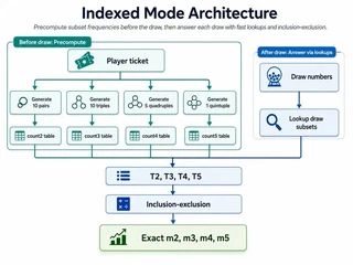
The indexed solution starts from a different question: can we move almost all of the work before the draw? Each ticket has five numbers, and from those five we can generate every smaller combination:

C(5,2) = 10 pairs
C(5,3) = 10 triples
C(5,4) =  5 quadruples
C(5,5) =  1 quintuple

For every ticket, during preprocessing, we increment a frequency counter for each of those subsets. For the ticket 1 2 3 4 5, the ten pairs (1,2) (1,3) (1,4) (1,5) (2,3) (2,4) (2,5) (3,4) (3,5) (4,5) each get bumped — and likewise for its triples, quadruples, and the full quintuple.

After preprocessing, when the draw arrives, we do not touch the player list at all. We generate the draw’s own 10 pairs, 10 triples, 5 quadruples, and 1 quintuple, and look each of them up in the precomputed tables. That is just 26 lookups, so the per-draw complexity is O(1) — it no longer depends on the number of players.

Scan mode asks: “which players match this draw?” Indexed mode asks: “how many tickets already contain each subset of this draw?”

Dense arrays instead of hash maps

A straightforward implementation might reach for hash maps. But here the universe is small and fixed — numbers are always 1 to 90 — so the number of possible combinations is finite, predictable, and small enough to store densely:

C(90,2) =      4,005
C(90,3) =    117,480
C(90,4) =  2,555,190
C(90,5) = 43,949,268

With 32-bit counters:
  count2:      4,005 × 4 B  ≈  16 KB
  count3:    117,480 × 4 B  ≈ 470 KB
  count4:  2,555,190 × 4 B  ≈  10 MB
  count5: 43,949,268 × 4 B  ≈ 176 MB
  ───────────────────────────────────
  total index memory        ≈ 186 MB

That is a reasonable price for constant-time queries, and dense arrays avoid hashing, bucket overhead, pointer chasing, allocation, and GC pressure. The only remaining puzzle is mapping each combination to a unique array index.

Ranking combinations with combinadics

Each combination needs a deterministic rank. Convert numbers to zero-based first (1..90 → 0..89), then for a sorted combination c0 < c1 < … < c(k-1) compute:

rank = C(c0,1) + C(c1,2) + ... + C(c(k-1),k)

For a 5-number combination:
rank = C(c0,1) + C(c1,2) + C(c2,3) + C(c3,4) + C(c4,5)Example — combination 1 2 3 4 5, zero-based 0 1 2 3 4:
rank = C(0,1) + C(1,2) + C(2,3) + C(3,4) + C(4,5)  →  a unique index into count5[]

The rank becomes the array index, and you write count5[rank]++. No maps, no serialized keys, no per-combination heap allocation — just direct counter increments. The binomial coefficients are themselves precomputed once with Pascal’s rule, so ranking never does arithmetic heavier than a few array reads and adds:

var binomial [91][6]uint64                 // binomial[n][r] = C(n,r)

func initBinomialTable() {
    for n := 0; n <= 90; n++ {
        binomial[n][0] = 1
        for r := 1; r <= 5; r++ {
            if r > n { binomial[n][r] = 0; continue }
            binomial[n][r] = binomial[n-1][r-1] + binomial[n-1][r]
        }
    }
}// rank of a sorted, zero-based quintuple c0<c1<c2<c3<c4:
rank := binomial[c0][1] + binomial[c1][2] + binomial[c2][3] +
        binomial[c3][4] + binomial[c4][5]   // lands in [0, C(90,5))

For a fixed, small combination space, this is exactly the transformation that turns a general-purpose solution into a high-performance one.

The subtle part: exact match counts

The indexed approach has one important trap — the bug that bit me in Iteration 3. The raw subset counts are not the final answer. A ticket matching all five drawn numbers contains 10 pairs, 10 triples, 5 quadruples, and 1 quintuple, so naively summing pair, triple, and quadruple totals counts it many times over. A four-match ticket similarly contributes 6 pairs, 4 triples, 1 quadruple.

The precomputed tables answer “how many tickets contain this pair/triple/quadruple?” But the business wants “how many tickets have exactly 2, 3, 4, or 5 matches?” Those are different questions, and conflating them is the most common bug in combination-indexed solutions.

From subset totals to exact counts

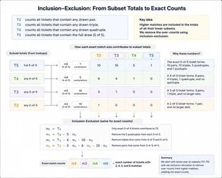
Let T2, T3, T4, T5 be the subset totals for the draw, and m2, m3, m4, m5 the exact match counts we want. Counting how each exact category contributes to each total:

Exactly 2 matches:  C(2,2)=1 pair
Exactly 3 matches:  C(3,2)=3 pairs,  C(3,3)=1 triple
Exactly 4 matches:  C(4,2)=6 pairs,  C(4,3)=4 triples, C(4,4)=1 quad
Exactly 5 matches:  C(5,2)=10 pairs, C(5,3)=10 triples, C(5,4)=5 quads, C(5,5)=1 quint

So the totals expand as:
  T5 = m5
  T4 = m4 + 5·m5
  T3 = m3 + 4·m4 + 10·m5
  T2 = m2 + 3·m3 + 6·m4 + 10·m5And we solve backward:
  m5 = T5
  m4 = T4 - 5·m5
  m3 = T3 - 4·m4 - 10·m5
  m2 = T2 - 3·m3 - 6·m4 - 10·m5

This is the core correction step. Without it, the indexed solution reports inflated counts — a fast wrong answer, which is just a more expensive bug.

Why the query is constant time

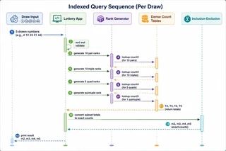
Put it together and the post-draw path is fixed work: generate 10 pairs, 10 triples, 5 quadruples, 1 quintuple; do 26 dense-array lookups to get T2–T5; apply the inclusion–exclusion correction; print. Whether there are 10,000 players, 10 million, or 100 million, the draw performs the same amount of work. In code, the entire correction is four lines — and the subset totals accumulate into int64 even though each stored count is a uint32, because a sum of subset totals can run larger than any single count:

// total2..total5 are int64 sums of the 26 looked-up counts
winners5 = int(total5)
winners4 = int(total4) - 5*winners5
winners3 = int(total3) - 4*winners4 - 10*winners5
winners2 = int(total2) - 3*winners3 - 6*winners4 - 10*winners5

Building the index without melting the cache

Here is the part the math never warns you about. On paper, preprocessing is trivial: for each player, bump 26 counters — ten million players, 260 million increments, done. So you write the obvious parallel loop, split the players across four cores, let each core increment the shared tables… and your beautiful O(1) query now sits behind a build that crawls, because four cores are elbowing each other for the same handful of cache lines.

The culprit is contention, and it is wildly uneven across the four tables. The pair table has only 4,005 slots but absorbs roughly 100 million increments, so a few cache lines run white-hot — atomic adds there would serialize the entire build on them. The quintuple table is the opposite: 44 million slots sharing only ~10 million increments, so collisions are rare. One strategy cannot be right for both, and the real code splits accordingly:

// SMALL + HOT (pairs: 4,005 slots, ~100M hits; triples: 117,480 slots):
// each worker counts into a PRIVATE copy, merged by index shard afterward.
local.pairs[binomial[a][1]+binomial[b][2]]++

// LARGE + SPARSE (quads: 2.5M slots; quintuples: 44M slots):
// atomic adds straight into the shared table — collisions are rare, and
// cloning 176 MB per worker would be absurd.
atomic.AddUint32(&quintupleCounts[rank], 1)

So the two small tables get per-worker private copies (zero contention while counting, then a quick shard-by-index-range merge), while the two big tables take atomic increments directly into shared memory (no 10 MB-and-176 MB-per-core duplication, and no merge pass at all). The payoff: a build whose peak memory stays roughly flat as cores are added, doing genuinely O(N) work with an O(N/p) span — no rescanning the dataset once per worker.

The lesson hiding in the build

The algorithm said “increment 26 counters.” The hardware said “watch four cores fight over one cache line.” Choosing private-accumulate versus atomic per table, by size and collision rate, is exactly the kind of decision the AI and I traded notes on — and exactly the kind that never survives into the tidy final write-up. Concurrency correctness is cheap to state and expensive to earn.

Why the indexed solution is not new mathematics

It is worth emphasizing, partly out of honesty and partly because it is the most reusable lesson here, that the indexed solution invents nothing. It is a composition of four classical results, none original to it — and they span more than a century.

1 · The addressing layer — the combinatorial number system (combinadics)

Representing each sorted k-combination as C(c₁,1) + C(c₂,2) + … + C(c_k,k) creates a bijection onto {0, …, C(n,k)−1}. The idea was observed by D. H. Lehmer (1964), later named the combinatorial number system by Donald Knuth in The Art of Computer Programming, Volume 4A (2011), who traces the underlying concept back to Ernesto Pascal (1887).

2 · The arithmetic — binomial coefficients

Underneath the ranking is nothing more exotic than C(n,k) = C(n−1,k−1) + C(n−1,k), commonly associated with Blaise Pascal (1654) though known much earlier in India, Persia, and China. Precomputing this triangle is what makes ranking allocation-free and fast.

3 · The counting layer — itemset support counting

Incrementing a counter for every subset contained in every record is essentially itemset support counting, the core idea behind the Apriori algorithm introduced by Rakesh Agrawal and Ramakrishnan Srikant (1994). Our “tickets” are transactions; our “combinations” are itemsets.

4 · The recovery layer — inclusion–exclusion (exactly-k)

Recovering exact winner counts from subset totals uses the exactly-k form of inclusion–exclusion:

m_j = Σ_{k≥j} (−1)^{k−j} · C(k,j) · T_k

This is associated with Charles Jordan, later generalized through the Schuette–Nesbitt formula, all resting on the classical inclusion–exclusion principle.

The actual contribution

The solution’s only original move is noticing these four pieces snap together in a way that makes query cost independent of dataset size. That is engineering, not new mathematics — and recognizing such compositions is precisely where an AI collaborator earns its keep, provided you supply the constraints that force the pieces into place.

Loading and parsing efficiently

For a 10-million-ticket dataset, parsing can dominate startup time. The input is ASCII text, one ticket per line (4 16 22 35 78, 1 2 3 4 5, …). A naive parser using high-level string splitting and per-line integer parsing is fine for small files but creates real overhead at scale: temporary strings, repeated allocation, expensive conversions, GC pressure.

Memory-map the file. Rather than copying the ~145 MB into a heap-owned slice the way os.ReadFile would, the file is mmap’d read-only: the OS faults pages in straight from its cache, in parallel, as the workers touch them — less heap pressure and free cooperation with the page cache (with a plain-read fallback when mapping is unavailable). Because parsing is the dominant cost, wall-clock load time then scales down roughly linearly with core count.

Split work by line boundaries. Parsing can run in parallel, but chunks must never split a ticket line. So the file is divided into byte ranges and each boundary is nudged forward to the next newline, guaranteeing every worker parses complete lines and writes to its own output buffer with no shared writes:

File bytes
┌──────────────────────────────────────────────────────────────┐
│ line line line line line line line line line line line line   │
└──────────────────────────────────────────────────────────────┘
          │                    │                    │
          ▼                    ▼                    ▼
   ┌────────────┐       ┌────────────┐       ┌────────────┐
   │ Worker 0   │       │ Worker 1   │       │ Worker 2   │
   │ whole lines │       │ whole lines │       │ whole lines │
   └────────────┘       └────────────┘       └────────────┘

Each worker emits its own packed buffer; a prefix sum over the per-chunk sizes hands every chunk a disjoint offset in the final slice, so the buffers are stitched together with a parallel copy and no worker ever overlaps another.

Then make the inner loop mean. Two small tricks keep the byte-level parse tight. A single unsigned subtraction decides whether a byte is a digit (if ch-'0' wraps above 9, it is not), and the running value is clamped while it accumulates, so an absurdly long token can never overflow an int and wrap back into the valid range — it is read in full, then rejected as out of range:

if ch-'0' > 9 {              // unsigned wrap-around: "is this a digit?"
    valid = false
}
// ...
if value <= maxNumber {      // clamp WHILE accumulating: no overflow, ever
    value = value*10 + int(digit)
}                            // 99999999999999999999 is read, then rejected

The output buffer is sized to a provably safe upper bound — a valid ticket consumes at least nine input bytes and emits five — so it appends without ever risking an overrun.

Validate while parsing. A valid ticket has exactly five distinct numbers in 1..90 — cheap to check. But validation policy is a product decision, not a performance one. Strict mode rejects the whole input if any line is malformed (right when every line is a real transaction); lenient mode skips bad lines and reports how many (useful for best-effort ingestion). Make the choice explicit — silent data loss is not an optimization.

Benchmarks & interpretation

I benchmarked both implementations on a deliberately constrained environment:

CPU:      4 logical CPUs used by the Go runtime
RAM:      4 GB
Go:       go1.23.2 linux/amd64
Setting:  GOMAXPROCS=4
Draws:    1 2 3 4 5  |  10 20 30 40 50  |  5 15 25 35 45
Metrics:  time-to-READY, per-draw latency, max RSS (/usr/bin/time -v)

A word on how the program runs, since it shapes what these numbers mean. It loads the file, prints READY, then reads draws from stdin and answers each on stdout, flushing per draw so the consumer gets every result immediately. Diagnostics go to stderr so the answer stream stays clean. Crucially, the per-draw timing brackets only the computation — not the line parsing or the printing — so a draw latency reflects the calculation itself, independent of I/O.

1 million players:

MODE      TIME→READY   DRAW1     DRAW2     DRAW3     AVG DRAW     MAX RSS
──────────────────────────────────────────────────────────────────────────
Scan       23.69 ms    0.884 ms  0.882 ms  0.915 ms  0.894 ms     40.5 MiB
Indexed   177.77 ms    1.472 µs  0.650 µs  0.628 µs  0.917 µs    202.9 MiB

At 1M players, scan mode is already fast enough — but indexed mode answers roughly three orders of magnitude faster per draw, in exchange for more time before READY and more memory.

10 million players:

MODE      TIME→READY   DRAW1      DRAW2       DRAW3       AVG DRAW    MAX RSS
──────────────────────────────────────────────────────────────────────────────
Scan      210.64 ms    7.978 ms   15.017 ms   13.687 ms   12.227 ms   255.9 MiB
Indexed    1.220 s     2.649 µs    1.044 µs    0.791 µs    1.495 µs   301.5 MiB

At 10M players, scan mode still performs well because it is streaming compact contiguous memory across four cores — an average of about 12.2 ms is very respectable. But indexed mode is in a different class, answering in about 1.5 µs after the index is built. The difference is simply: scan touches every ticket after the draw; indexed touches 26 counters.

Putting the gap on a bar

10 million players · average draw latency

Scan mode     12.227 ms  ██████████████████████████████████████████████████
Indexed mode   0.0015 ms  ▏ratio ≈ 12.227 ms / 0.001495 ms ≈ 8,178×

So indexed mode was roughly 8,000× faster per draw here. That does not make scan mode bad — it means the two modes optimize different parts of the system.

Startup vs. query latency (the break-even)

10 million players
  Scan:     before READY ~211 ms   |  per draw ~12 ms
  Indexed:  before READY ~1.22 s   |  per draw ~1.5 µs

extra startup cost of indexed   = 1.220 s − 0.211 s ≈ 1.009 s
per-draw saving                 = 12.227 ms − 0.0015 ms ≈ 12.2255 ms
break-even                      = 1.009 s / 12.2255 ms ≈ 83 draws

If you only care about total runtime on this machine and dataset, indexed mode pays back its extra preprocessing after about 83 draws. But total runtime is often the wrong metric: if the requirement is minimum latency after the draw, indexed mode is justified even for a single draw, because it moves work out of the critical path.

On memory: measured max RSS was ~256 MiB (scan) and ~302 MiB (indexed). The theoretical tables are ~186 MB plus ~50 MB of packed tickets; measured RSS also includes runtime overhead and mapped pages, so it will not match exactly. One small but deliberate touch: once the indexed tables are built, the program drops the ~50 MB ticket buffer (packedTickets = nil) and forces a GC, since indexed draws read only the tables — keeping steady-state memory closer to the tables themselves. Both modes fit comfortably in 4 GB.

Comparing the two approaches

DIMENSION                  SCAN MODE                 INDEXED MODE
────────────────────────────────────────────────────────────────────────────
Preprocessing              minimal                   heavier
Per-draw complexity        O(N)                      O(1)
Memory usage               lower                     higher
Implementation complexity  lower                     higher
Scaling with players       linear per draw           constant per draw
Debuggability              very high                 requires stronger validation
Best use case              low memory, baseline      lowest post-draw latency

Choose scan mode when memory is constrained, the dataset is modest, draws are rare, or you want a correctness baseline. Choose indexed mode when post-draw latency is critical, there may be many queries, the player count may grow, and enough memory is available. Indexed mode is not “better” in every dimension — only for the one goal of minimizing critical-path latency. That is the engineering tradeoff.

Performance lessons from this problem

The Hungarian lottery problem is small, but it demonstrates several principles that apply to many performance-heavy systems.

1. Optimize the critical path

The critical path is the work that must happen while someone is waiting.

Here, that is the post-draw report.

Indexing is valuable because it moves work from the critical path into the preparation phase.

This pattern appears everywhere:

• search engines build inverted indexes before queries
• databases maintain indexes before reads
• compilers build intermediate representations before optimization
• recommendation systems precompute features before serving
• analytics systems aggregate data before dashboard queries

Precomputation is not an implementation detail.

It is a latency strategy.

2. Data layout matters

The scan solution is fast because the data layout is simple and compact.

A flat byte array is not glamorous, but it works well.

Many performance problems are not solved by more abstraction. They are solved by fewer cache misses.

Before optimizing arithmetic, look at memory access patterns.

3. Avoid allocations in hot paths

The draw path should not allocate per ticket.

The indexed query path should not allocate per combination.

The parser should avoid temporary strings where possible.

Allocation is not always expensive, but repeated allocation in hot paths creates secondary costs:

• allocator overhead
• garbage collection
• memory fragmentation
• reduced locality

4. Measure phases separately

A single “total runtime” number can be misleading.

For this problem, scan mode may start faster, while indexed mode answers faster.

Neither number alone tells the full story.

Performance-heavy systems usually have multiple important latencies:

• cold start
• warm query
• p50 latency
• p99 latency
• peak memory
• throughput
• tail behavior under concurrency

Measure what matters.

5. Keep a simple implementation around

The scan implementation is useful even when indexed mode is the default.

It helps validate correctness.

It provides a fallback.

It gives future engineers a simpler mental model.

In high-performance systems, complexity tends to accumulate. A clear baseline keeps the project grounded.

6. Exact semantics matter

The indexed solution’s biggest risk is not performance.

It is semantics.

Subset counts are not exact match counts.

That difference is easy to miss, and it completely changes the answer.

Performance work must never blur the meaning of the result.

A fast wrong answer is just a more expensive bug.

Closing thoughts

This problem starts as a lottery-counting exercise, but it quickly becomes a performance engineering problem.

The core lesson is not specific to lotteries.

The broader lesson is:

Move work out of the critical path when the problem allows it.

The scan solution shows how far careful data layout and a simple CPU-friendly loop can go.

The indexed solution shows how preprocessing can change the runtime model completely.

On a 4 CPU / 4 GB RAM environment, scan mode handled 10 million players with an average draw latency of about 12 ms. That is already very fast.

Indexed mode handled the same 10 million players with an average draw latency of about 1.5 microseconds after preprocessing.

The Bottom Line

Ultimately, software engineering rarely hands us a single “correct” path only trade-offs. Both solutions are incredibly valuable; they simply optimize for entirely different dimensions of performance.

• Sometimes, the right answer is minimalist: a flat array paired with a tight, cache-friendly loop for raw speed.
• Sometimes, the right answer is structural: a precomputed index that slashes lookup times as complexity scales.

The most resilient architectures don’t treat these patterns as rivals. They recognize that the best system often doesn’t force a choice between the two, it harmoniously leverages both.